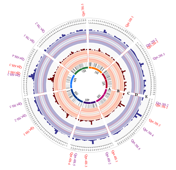
An interactive Circos plot indicating QTL involved in net blotch resistance and displayed using histogram, arc, link, background, text function.
Normally, the SNP data is stored in .vcf format, thus we use an real VCF file as example here.
The example of real SNP file is available here
First, we need to extract the effective SNP columns from the original VCF file
# Load original SNP data
library(interacCircos)
library(stringr)

SNP_data<-read.table("snpExample_random_from_1000G.vcf",sep = "\t")
SNP_data<-SNP_data[,c(1,2,8)]
colnames(SNP_data)<-c("chr","pos","value")
SNP_data$value<-as.integer(str_split_fixed(str_split_fixed(SNP_data$value,
 ";", 2)[,1],"=",2)[,2])
After processing, the SNP_data should looks like below:
| chr | pos | value |
|---|---|---|
| 1 | 70573281 | 9 |
| 1 | 167102542 | 1 |
| 1 | 238165263 | 1 |
| 2 | 52714177 | 1827 |
| ... | ... | ... |
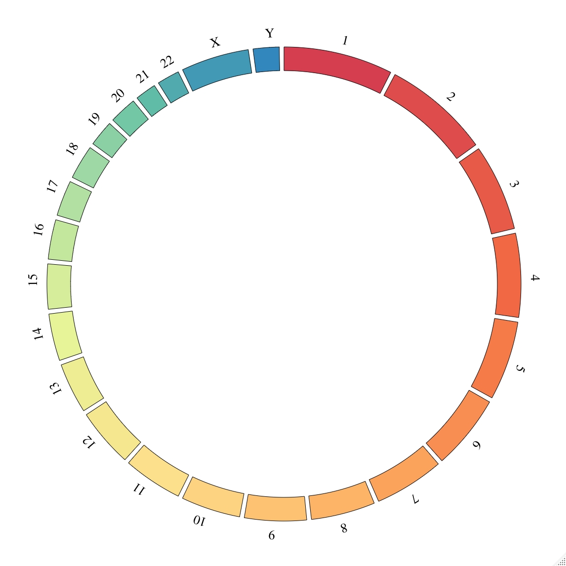
In order to load other functional tracks, users should first construct a chromosome track!
# Load original SNP data
library(interacCircos)
library(stringr)

SNP_data<-read.table("snpExample_random_from_1000G.vcf",sep = "\t")
SNP_data<-SNP_data[,c(1,2,8)]
colnames(SNP_data)<-c("chr","pos","value")
SNP_data$value<-as.integer(str_split_fixed(str_split_fixed(SNP_data$value,
 ";", 2)[,1],"=",2)[,2])

Circos()
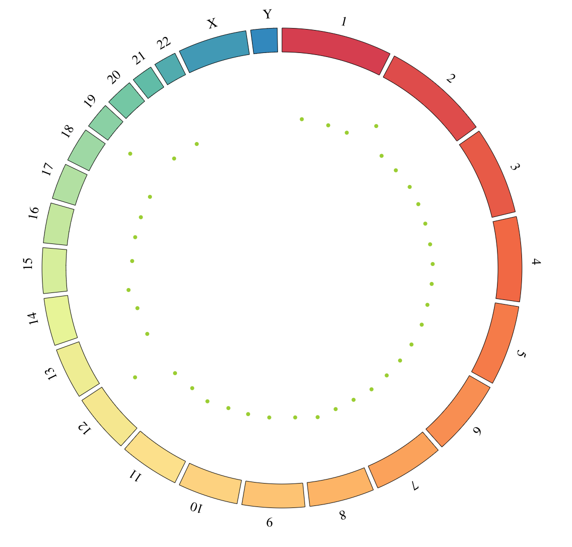
In order to add snp track, users should first constrct a CircosSNP() function and then load this track on Circos() function
# Load original SNP data
library(interacCircos)
library(stringr)

SNP_data<-read.table("snpExample_random_from_1000G.vcf",sep = "\t")
SNP_data<-SNP_data[,c(1,2,8)]
colnames(SNP_data)<-c("chr","pos","value")
SNP_data$value<-as.integer(str_split_fixed(str_split_fixed(SNP_data$value, ";", 2)[,1],"=",2)[,2])

SNP_track<-CircosSnp('SNP01', minRadius =150, maxRadius = 190, data = SNP_data,fillColor= "#9ACD32",
                                      circleSize= 2)

Circos(moduleList = SNP_track)
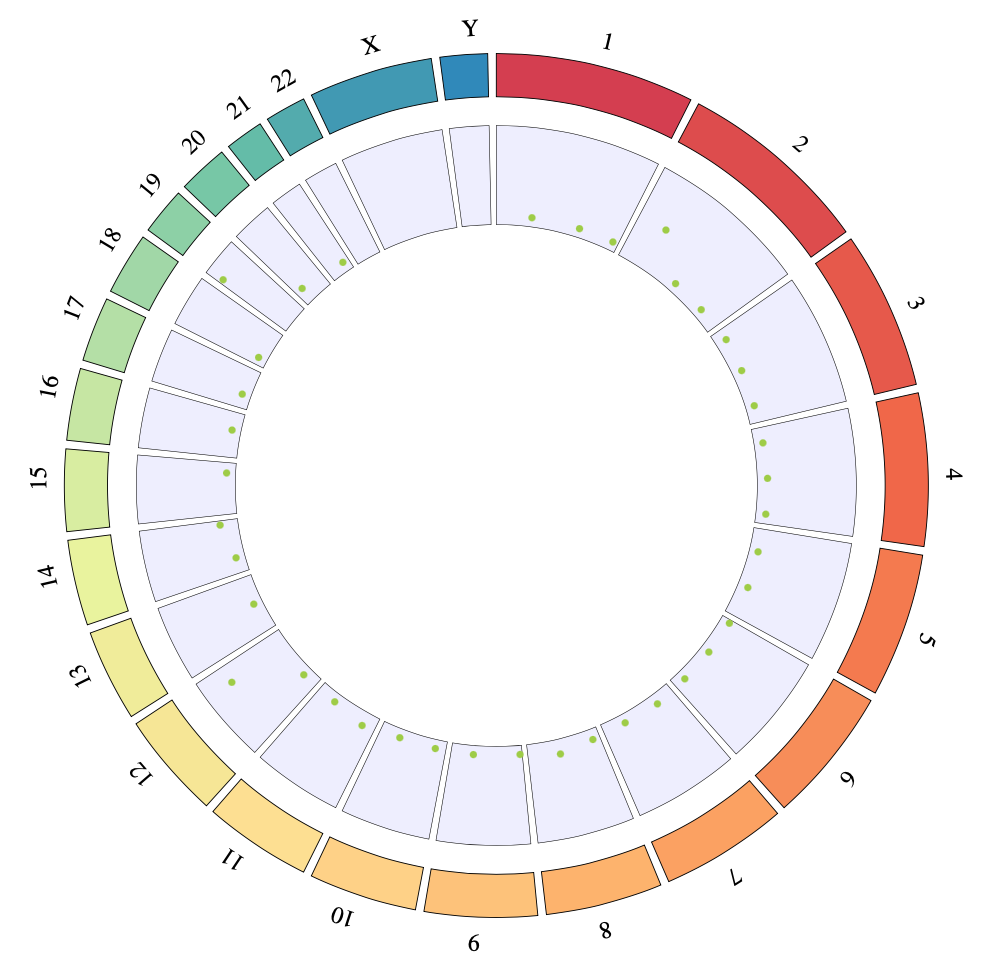
It's not pretty enough when only add a snp track, users can add other tracks to increase readability.
# Load original SNP data
library(interacCircos)
library(stringr)

SNP_data<-read.table("snpExample_random_from_1000G.vcf",sep = "\t")
SNP_data<-SNP_data[,c(1,2,8)]
colnames(SNP_data)<-c("chr","pos","value")
SNP_data$value<-as.integer(str_split_fixed(str_split_fixed(SNP_data$value, ";", 2)[,1],"=",2)[,2])

SNP_track<-CircosSnp('SNP01', minRadius =150, maxRadius = 190, data = SNP_data,fillColor= "#9ACD32",
                                      circleSize= 2)
Bg_track<-CircosBackground('BG01',minRadius = 145, maxRadius = 200)

Circos(moduleList = SNP_track+Bg_track)
As you know, interacCircos is interactive as it can add animation and mouse event to plot. Here, we add a mouse move event and a opening animation for snp track
# Load original SNP data
library(interacCircos)
library(stringr)

SNP_data<-read.table("snpExample_random_from_1000G.vcf",sep = "\t")
SNP_data<-SNP_data[,c(1,2,8)]
colnames(SNP_data)<-c("chr","pos","value")
SNP_data$value<-as.integer(str_split_fixed(str_split_fixed(SNP_data$value, ";", 2)[,1],"=",2)[,2])

SNP_track<-CircosSnp('SNP01', minRadius =150, maxRadius = 190, data = SNP_data,fillColor= "#9ACD32",
                                      circleSize= 2, animationDisplay =TRUE,animationTime= 2000,animationDelay= 0,
                                      animationType= "linear")
Bg_track<-CircosBackground('BG01',minRadius = 145, maxRadius = 200)

Circos(moduleList = SNP_track+Bg_track,SNPMouseEvent = TRUE,SNPMouseOverDisplay = TRUE,
SNPMouseOverTooltipsSetting = "style1",SNPMouseOutDisplay = TRUE,SNPMouseOutColor = NULL)
An interactive Circos plot indicating QTL involved in net blotch resistance and displayed using histogram, arc, link, background, text function.
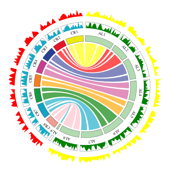
An interactive Circos plot displaying the comparative genomic mapping in C. rubella(CR), A. lyrata(AL) and displayed using chord, wig, background function.
I'm a PhD student at Harbin Institute of Technology working on genome visualization and single cell ATAC sequencing.
If you have any questions about interacCircos, you are very welcome to contact me through github or email.
If you are interested in our lab, you are very welcome to visit our website!